Authors:
(1) Tinghui Ouyang, National Institute of Informatics, Japan ([email protected]);
(2) Isao Echizen, National Institute of Informatics, Japan ([email protected]);
(3) Yoshiki Seo, Digital Architecture Research Center, National Institute of Advanced Industrial Science and Technology, Japan ([email protected]).
Table of Links
Description and Related Work of OOD Detection
Conclusions, Acknowledgement and References
III. METHODOLOGY
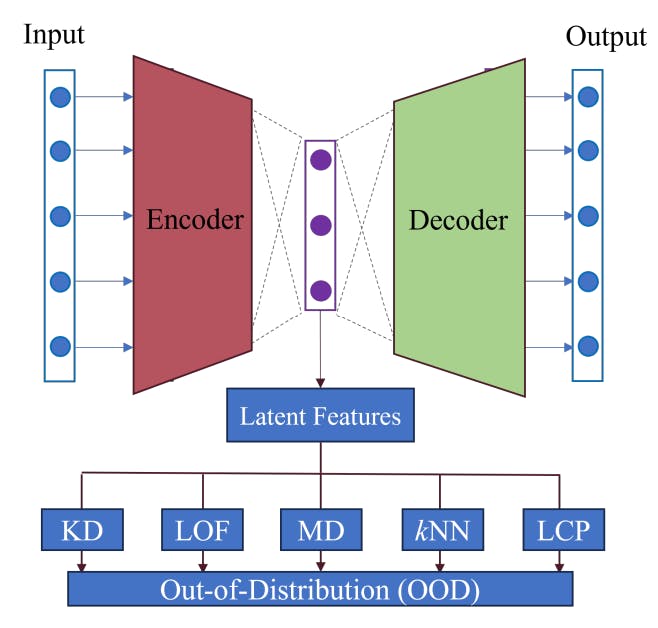
From the above description in Section II, the core idea of OOD detection is to use statistical measure, e.g., distribution probability or structural characteristics (distance and density), to distinguish normal and outlier data. However, in terms of complex and high-dimensional data, data’s distribution and structural characteristics are not as apparent as that of low-dimensional data. In this case, data transformation is required to simplify data. Therefore, this paper proposes a general framework of the OOD detection method via statistical measures in Fig. 2.

Fig. 2 shows the framework of the proposed OOD detection method, which makes use of statistical measures as the score function in (1), then determines outlier or normal data. Considering the structural characteristics of high-dimensional data are not readily computed, so a deep AE architecture is used for feature learning and dimensionality reduction first, as shown in Fig. 2. Then, some conventional statistical measures are used to calculate the OOD score based on this framework. In this paper, a new statistical measure for better OOD description and detection performance is also come up with, namely the LCP measure in Fig. 2. Details for its implementation are described as follows.
A. activation traces
As mentioned, the proposed framework utilizes deep AE for feature learning and dimensionality reduction. Considering normal and outlier data may have different neuron behaviours in deep learning, this paper proposes to use latent features’ neuron activation status for better OOD study instead of original data. This idea is inspired by [20], which proposed that using neurons’ status with respect to a testing data point is a good way to describe data’s behavior. For example, the neuron’s activation value is one of the most straightforward descriptions of data behaviors with respect to the given DL model, as well as the sign of neuron outputs. Then, based on these activation statuses, some neuron coverage metrics [21] were defined to describe the data’s behaviors. In this paper, we can simply define the activation values as the trace of neuron behavior.
By assuming a given deep learning architecture consisting of a set of neurons N = {n1, n2, · · · }, then, for a given testing data x ∈ {X|x1, x2, · · · }, its activation trace with respect to Ncan be defined as A(x) = σN (x). Generally, considering a DL model contains a huge number of neurons, it is more effective to calculate the activation trace of an ordered (sub)set of neurons Ns ⊆ N, instead of all neurons. Inspired by the paper [22], which demonstrates abnormal and normal data have different neuron activation statuses on the information channel and the activation network, this paper considers choosing the most active neurons in testing in order to reduce feature dimensionality and computation cost. Moreover, according to the description of the proposed framework, an AE architecture is used for feature representation from high-dimensional and complex data space to low-dimensional space. AEs have the advantage of learning the most representative features with low rank so that they can preserve important information of original data in the dimensionality reduction process. Therefore, the activation traces of active neurons in the latent space of AE are calculated as the features for OOD detection in accordance with the proposed framework in Fig. 2.
B. local conditional probability (LCP)
Then, based on the data’s features of activation trace, different statistical measures are applied to calculate the OOD data score, like KD, MD, kNN, and LOF in Fig. 2. However, summarizing these measures, it is found that the main ideas of these methods are to leverage the average distance as the representation of probability or density in OOD scoring. For example, KD uses the average kernel distances from the global dataset, MD to calculate the Mahanalobis distance. Unlike KD and MD, kNN calculates the average Euclidean distance in a local neighborhood domain. Even though LOF is totally different from the other methods, it also makes use of local neighbors’ information, namely the average reachability in the OOD score definition. With consideration of effectiveness of these methods in OOD detection, this paper propose to combine both neighborhood information and distance to develop a statistical measurement for OOD scoring.
Firstly, instead of calculating the average distance, this paper proposes to reconstruct the testing data via a linear combination of the given training data and then calculate the reconstruction distance as the final OOD score, as defined below

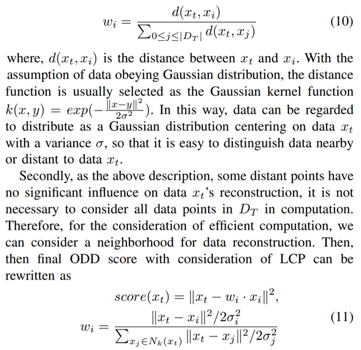
where wi is the weight for each individual data point xi . It is known that this reconstruction idea is also a useful strategy in OOD detection and shares some similar concepts with that of the distance-based method. For example, KD and kNN can also be regarded to calculate the distance between the testing data xt and the center of the whole data and neighbors, respectively. The wi can be thought of as equal weights in KD/kNN even though they are not for reconstruction. However, with consideration of data reconstruction, the weights wi should be specified to well reproduce the testing data P xt and satisfy wi = 1. Therefore, a kind of similarity based on local conditional probability (LCP) is defined as the weights in this paper, as below

Moreover, considering the distances between two points vary a lot and have different effects on the Gaussian kernel, so the value of σ in this paper is considered to be selected based on the binary search method in [25].
This paper is available on arxiv under CC 4.0 license.

